LB simulation of 3D spinodal decomposition in the inertial regime

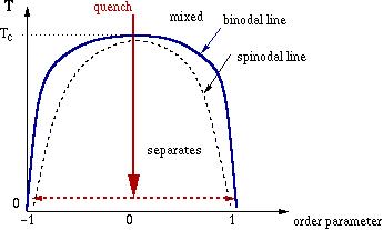
When an incompressible binary fluid mixture is quenched far below its spinodal temperature, it will phase separate into domains of the two fluids.

Here we study the simplest case - two fluids A and B have identical properties in all respects except that they are mutually phobic - and a deep quench so thermodynamic equilibrium has the two fluids completely demixed.

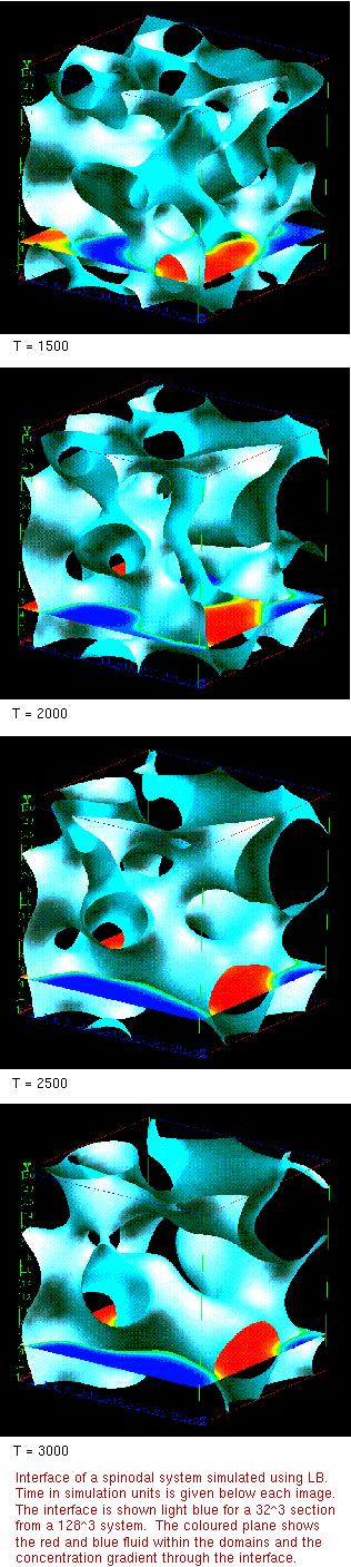
For a 50-50 mixture the two fluids form an interlocking structure as they separate. Shown in the diagram on the right is the interface between them at successive times, the interface is light blue, and the coloured plane shows the red/blue fluid within the domains.

The late-stage growth is driven by capillary forces (Laplace pressure), arising from curvature of the (sharply defined) interface between the two fluids; these drive fluid flows from regions of tight curvature (necks, narrow liquid bridges) into those of low interfacial curvature (large domains).

Note that for coarsening of a bicontinuous structure to proceed this way, one also requires discrete ``pinch-off" events to continually occur: each of these allows the topology to change discontinuously in time. In the picture for time T=3000 (simulation units), a neck close to breaking point can be seen towards the upper left of the image.

Besides the relative concentrations of the two fluids (50-50) and the quench depth, the other significant parameters are the surface tension, , the viscosity, , and the fluid mass density, , There is also a mobility parameter, , which controls the diffusion.

More details of this work can be found in[Kendon et al.(1999)].

(Return to top.)

This simple system is modeled by a pair of coupled differential equations for the fluid velocity and fluid composition. The fluid velocity obeys the Navier-Stokes equation with a forcing term from the interface, which moves the fluid around as it straightens and shrinks. The fluid composition is modeled as the difference in density between the two fluids, , which plays the role of the order parameter, and evolves via a convection diffusion equation in which convection is provided by the fluid velocity.

The free energy, F, for the system is chosen to have a double well potential with parameters determined so as to cause sharp interfaces to form,

F = dr - A ² + B ⁴ + k( )² + 1/3 ln .

Parameters A and B control the shape and depth of the double well, while k determines the interfacial tension between the two fluids. The interface width is about 6 , where ² = k/2A.

(Return to top.)

Given the above model, theory says that there should be three distinct, universal growth regions[Bray(1994)] for the average domain size, L:

• diffusive: L T^1/3 for L ( )^1/2 ( = molecular scale)
  
• viscous hydrodynamic: L T for ( )^1/2 L
  
• inertial: L T^2/3 for L
  

is a crossover length between the viscous hydrodynamic region, where viscous drag is the main resistance to the driving force, to the inertial region where finite Reynold's number effects come into play. Theory predicts that

where is the surface tension.

A prediction of a further crossover to a scaling in which L scales as T^1/2 was made recently [Grant and Elder(1999)]. The argument is that turbulence will develop as the system coarsens further into the inertial region, and this will eventually remix the fluids by disrupting the interface, slowing down the growth still further from T^2/3.

(Return to top.)

In order to compare different simulations in a meaningful, universal way, we need to use length and time scales based on the physical parameters of the system. For given values of , and , it is possible to form a characteristic length,

and a characteristic time,

Using L₀ and T₀ as the units of length and time, the scaling equations become,

A useful non-dimensional measure used to characterise fluid systems is the Reynolds number, Re, defined as (velocity x length)/(kinematic viscosity). For this system, the obvious choices of typical length and velocity are L and dL/dT, giving Re = L dL/dT, since in these scaled units, with fluid density, = 1, the viscosity is equal to 1. The Reynolds number gives an estimate of the ratio of the nonlinear term in the Navier-Stokes equation, (v. )v, to the viscous term, ²v, where v is the fluid velocity.

(Return to top.)

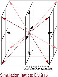
The above model equations have been simulated using a Lattice Boltzmann (LB) method, on a D3Q15 lattice (see diagram, right). For details of the method, see[Swift et al.(1996)]; details of the code will appear in[Bladon and Desplat].

The simulations were run on the two of the parallel computers at the Edinburgh Parallel Computing Centre, a Cray T3D and a Hitachi SR-2201. The largest system size was 256³, using 256 processors on the T3D, and producing around 4Gb of output data in the form of order parameter and velocity fields coarse-grained down to 128³.

The LB method allows the values of the viscosity, surface tension, fluid density, interface width and mobility (diffusion) to be set; careful choice of these parameters is necessary to ensure that the simulation

• remains stable through late times,
• maintains the interface profile in local equilibrium,
• limits the direct contribution from diffusion to the domain growth to negligible values in the region of interest.

The order parameter data was analysed to extract a length scale using Fourier transforms to obtain the first moment of the spherically averaged structure factor.

The velocity field was also analysed using Fourier transforms to compute derivatives, in order to compare the magnitude of the viscous and inertial terms in the Navier-Stokes equation, and measure the skewness of the longitudinal velocity derivatives.

(Return to top.)

For each simulation run, the measured lengths (obtained from the order parameter data) and times have been scaled using L₀ and T₀ to form a single universal graph of domain growth. (Also, in order to focus on the viscous and inertial regions, any offset due to an initial diffusive period has been subtracted.) This enabled all of the main data runs to be displayed on a single log-log plot, see below, covering five decades of reduced length and seven decades of reduced time.

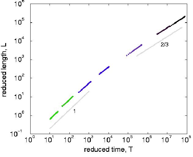
The eight main LB runs cover a linear region 1 < T < 10², a long crossover region, 10² < T < 10⁶ and an inertial region 10⁶ < T < 10⁸, so the predicted scaling behaviour is observed in our results.

No single run could cover the range of length and time scales presented here, for that a simulation grid of around a million cubed would be required, run for around 10¹⁰ time steps.

This is the first time the inertial region has been clearly observed in simulation, see[Kendon et al.(1999)] for discussion of other related work.

(Return to top.)

Since there are many factors that could produce a scaling that appears to be T^2/3, we made a number of checks to make sure that our observed results really are due to the simulation being in the inertial region, and further, to see if the inertial nature of the fluid was leading to the development of turbulence:

• we calculated the growth rate due to diffusion and then ensured that data was only used for the final graph (above) if the diffusive growth was under 2% of the total growth rate.

• to avoid finite size effects due to the periodic boundary conditions causing the system to "interact with itself", an upper cut-off for the data used was set at one quarter of the system size.

• from the velocity field, the individual terms in the Navier-Stokes Equation were calculated, and the ratio of inertial to viscous terms compared for each run, showing that in the linear region the viscous term dominated over the inertial terms, and in the inertial region the reverse was true.

• the skewness of the longitudinal velocity derivatives was calculated - in turbulence this assumes a value of -0.5, in our most inertial run, a value of -0.35 was found, which is consistent with patches of turbulence developing within the domains, but not throughout the whole system. Visualisation of the interface shows that it is not disrupted by turbulent mixing, as might be the case if turbulence developed throughout the system.

We have used a Lattice-Boltzmann method to successfully simulate spinodal decomposition of a symetric, binary fluid mixture in the linear (viscous hydrodynamic) region, through a broad crossover to the inertial region where the domain size scales as T^2/3, the first time the inertial region has been unambiguously observed in simulation.

In the linear region, L < 1, with L=bT we find the universal constant, b, to have a value around b = 0.070 +/- 0.007.

This small value of b leads to the crossover region corresponding to large values of T of around 10² to 10⁶. Expressed in terms of Reynolds numbers, Re = L dL/dT, the crossover region does not appear so broad, occuring in the range 1 < Re < 100.

In the inertial region, T > 10⁶, with L=cT^2/3 the universal constant c is around c = 1.

We don't see any evidence for the prediction[Grant and Elder(1999)] of a further reduction in scaling exponent to a regime of domain size scaling as T^1/2, but this does not rule it out further into the inertial regime than we were able to simulate.

(Return to top.)

Kendon et al.(1999)

V M Kendon, J-C Desplat, P Bladon, and M E Cates. 3-D spinodal decomposition in the inertial regime. cond-mat/9902346, 1999.

Bray(1994)

A J Bray. Theory of phase-ordering kinetics. Adv. Phys., 43:-459, 1994.

Grant and Elder.

M Grant and K R Elder. Spinodal decomposition in fluids. Phys. Rev. Lett., 81:-14, 1999.

Swift et al.(1996)

M R Swift, E Orlandini, W R Osborn, and J Yeomans. Lattice Boltzmann simulations of liquid-gas and binary fluid systems. Phys. Rev. E, 54:-5052, 1996.

Bladon and Desplat.

P Bladon and J-C Desplat. Ludwig: A general purpose Lattice-Boltzmann code. in preparation.

Revision: 18th April 1999
(Return to top.)